Location of the hippocampus in the brain, anterior view. The hippocampus is located in the medial temporal lobe, and has been shown to be involved in memory and spatial navigation. Teal lines denote the hippocampus midline (medial core).

Subcortical Structure Shape Analysis Preprocessing Steps

The scripts described below may be used to perform surface deformation analyses on subcortical structures such as the hippocampus, thalamus, and the basal ganglia. Please email lhamilto[at]loni.ucla.edu with any questions or comments.

The Scripts

The scripts needed to perform the analysis are located at /cxfs/schizo/family_study/scripts/hippo_scripts/. It may be best if you copy these into your own scripts directory so that you may edit them to accommodate your own data set. Their names and order of execution are:

1. 3a_REDIG_RESLICE
2. 3b_avg.csh
3. 4a_make_core_ALL_CT_new.csh
4. get_vol.csh

Run all scripts on inire.loni.ucla.edu or autarch.loni.ucla.edu (older and slower).

3a_REDIG_RESLICE.csh

This script reslices and redigitizes all of your UCFs so that they all have the same number of levels and can be analyzed for surface deformation.

1. Change to the directory containing your UCFs.
2. Execute the script (which will look for any file matching *.ucf and will redigitize and reslice it, placing the resultant meshes into a subdirectory called MESHES. Resliced, redigitized files will have the prefix "RSP_".
   
   inire% cd /yourdirectory/HIPPO_UCFS/
   inire% /yourdirectory/scripts/3a_REDIG_RESLICE.csh
3. redigarb and reslicer in Paul's directory: /data/ad/mass3/users/PAULS_SURFACE_CODE/SGI/FIX/ will perform the redigitizing step and reslicing step, respectively. See Paul's webpage for more info on his code and scripts.
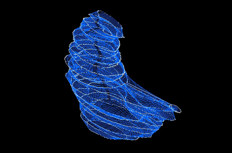
4. You will end up with a redigitized UCF that looks like the mesh below in blue (this sample shows the left thalamus). The white contours are the original traces from MultiTracer.
   
   

3b_avg.csh

This script simply creates an average and variance UCF for both the left and right hippocampi (or thalami, etc) so that you may investigate the average surface and variance over each point on the surface. You can change this script to make averages for all your patients or all your controls if you wish--just put the subjects of interest in their own directory and run from there.

5. Edit lines 8 and 9 in 3b_avg.csh so that RSP_*_HIPPO_${side}.ucf corresponds to the naming convention you are using in your processing stream. Also edit line 6 if you are naming sides using anything other than L and R (like LEFT or RIGHT).
6. Leave the ucf4d_to_dx lines commented out unless you wish to look at your UCFs in Data Explorer.
7. Run the script on inire from the same directory as before (containing your original UCFs):
   
   inire% cd /yourdirectory/HIPPO_UCFS
   inire% /yourdirectory/scripts/3b_avg.csh
8. surfNstat3D creates the average map, surfNstat4D creates the variance map.

4a_make_core_ALL_CT_new.csh

The 4a_make_core script is the last step before running statistics on your UCFs. This script generates a dist_core 4D UCF that encodes the distance from the medial core (running through the center of mass of the UCF) to the surface in the fourth column of the UCF. The resulting dist_core files may be used for surface deformation analysis in R.

9. Create a text file with a list of subject IDs for your analysis. Change line 9 so that `cat ../new_hippos.txt` opens this text file instead (i.e. `cat /mydir/hippo_subjs.txt`.
10. Change all instances of RSP_{$subj}_HIPPO_{$side}.ucf to reflect your naming convention. Note that other output files may be named RSP_core, dist_core, etc., and should be changed as well. (See lines 13, 15, 16, 20, 21, 23, and 30). Also change L and R if your files use LEFT and RIGHT or other naming conventions.
11. Run in the directory containing your UCFs, as before.
    
    inire% cd /yourdirectory/HIPPO_UCFS
    inire% /yourdirectory/scripts/4a_make_core_ALL_CT_new.csh
12. When this has finished, you should open your UCFs in nedit and make sure that the number of levels is correct. For the hippocampus, this is usually 150 levels, but the scripts may assume 255 levels, so be sure to edit this number if it is wrong. Your files will NOT load in ShapeViewer if the number of levels is not correct.
13. medial_core calculates the medial core through the UCF (basically a line running through the center of your meshes, orthogonal to the plane in which the contours were drawn). min_dist_onesurf_to_many creates a dist_core file which has the distance measure from each point on the RSP_ ucf to the medial core in the fourth column of the UCF. arb_surfNstat4D_avg4D_ucfs creates a 4D average of your UCFs. Again, you may wish to modify this line (30) to make separate averages for different groups.

get_vol.csh

This script can really be run at any time, as the files created do not depend on any files from the aforementioned scripts existing.

14. Change line 3 to be your analysis directory.
15. Change each of the foreach loops to cat your subject list text file (made for step 4).
16. Change the HIPPO_ANALYSIS directory to wherever you'd like your outputs to end up, and change family_study to the name of your project.
17. inire% /yourdirectory/scripts/getvol.csh

• Site Map ∗
• BMAP Home